Inelastic scattering
A fully rigorous method for including inelastic attenuation is so
far not available, and thus we use the common phenomenological
approach of an exponential decay of the amplitude of each
component of the photoelectron wave with the distance traveled
in the solid before escaping through the surface, called electron
inelastic mean free path (IMFP). If the distance traveled along a
given path is a and IMFP is
l, then the exponential decay factor
for the amplitude of this path is
exp(-a/(2l)).
Considering the inelastic scattering and vibrational effects,
we only need to rewrite eqn. (18) as follows:
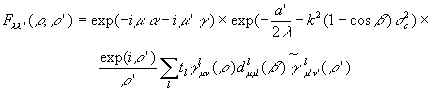
|
(26)
|
where a' is the internuclear distance of the bond vector leading
from the site in a single scattering process, see Figure 2.
sc2 is the thermal
mean square relative displacement, which will be discussed later.
The inelastic mean free path can be obtained from theory and
certain types of experiments. Tanuma, Powell and Penn have found
an empirical formula, called TPP-2 formula, to calculate IMFP
for 50-2000 eV electrons, based on the assumption that the Born
approximation is valid and on the neglect of vertex corrections,
self-consistency, exchange and correlation. The TPP-2 formula is

|
(27)
|
where l is the IMFP (in Å), E is the
electron energy (in eV), Ep=28.821(Nv
r/M)1/2 is the free-electron
plasmon energy (in eV), r
is the density of the bulk (in g.cm-3), Nv is
the number of valence electrons
per atom (for elements) or molecule (for compounds) and M is the
atomic or molecular weight. The terms b,
g, C and D are parameters given by
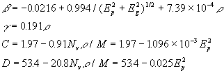
|
(28)
|
and Eg is the bandgap energy (in eV) for non-conductors,
and equals zero for conductors. The relationship of electron
energy E and wave number k is

|
(29)
|
Although there is no known physical basis, there is another
relatively simple and convenient means for expressing IMFP
dependence on electron energy, which was proposed by Wagner,
Davis and Riggs.

|
(30)
|
where k and m are material-dependent parameters. They found that m
ranged from 0.54 to 0.81. Generally, similar results have been
reported by others. Tables 2 and 3 list the empirical
parameters k and m for 27 elements and 15 inorganic compounds
over the electron energy range 500-2000 eV.
It appears from Tables 2 and 3 that
m=0.75±0.03 (one standard deviation) is a reasonable
approximation for this group of materials over 50-2000 eV.
| Element |
k |
m |
Element |
k |
m |
| C |
0.129 |
0.775 |
Ru |
0.0843 |
0.752 |
| Mg |
0.112 |
0.789 |
Rh |
0.0812 |
0.747 |
| Al |
0.0920 |
0.777 |
Pd |
0.104 |
0.748 |
| Si |
0.116 |
0.775 |
Ag |
0.0924 |
0.730 |
| Ti |
0.104 |
0.783 |
Hf |
0.156 |
0.719 |
| V |
0.0998 |
0.775 |
Ta |
0.104 |
0.720 |
| Cr |
0.0858 |
0.763 |
W |
0.0958 |
0.716 |
| Fe |
0.0897 |
0.753 |
Re |
0.0804 |
0.713 |
| Ni |
0.0942 |
0.734 |
Os |
0.0990 |
0.706 |
| Cu |
0.107 |
0.729 |
Ir |
0.104 |
0.708 |
| Y |
0.117 |
0.768 |
Pt |
0.0956 |
0.714 |
| Zr |
0.104 |
0.768 |
Au |
0.0951 |
0.713 |
| Nb |
0.132 |
0.745 |
Bi |
0.118 |
0.746 |
| Mo |
0.0941 |
0.748 |
|
|
|
| Table 2. Values of the parameters k and m in the fits of
eqn (30) to IMFPs calculated from experimental optical data for
27 elements over the electron energy range 500-2000 eV
|
| Compound |
k |
m |
Compound |
k |
m |
| Al2O3 |
0.122 |
0.750 |
NaCl |
0.192 |
0.760 |
| GaAs |
0.235 |
0.725 |
PbS |
0.121 |
0.765 |
| GaP |
0.144 |
0.755 |
PbTe |
0.114 |
0.771 |
| InAs |
0.192 |
0.736 |
SiC |
0.104 |
0.764 |
| InP |
0.0977 |
0.761 |
Si3N4 |
0.136 |
0.751 |
| InSb |
0.196 |
0.749 |
SiO2 |
0.150 |
0.764 |
| KCl |
0.169 |
0.769 |
ZnS |
0.145 |
0.752 |
| LiF |
0.127 |
0.764 |
|
|
|
| Table 3. Values of the parameters k and m in the fits of
eqn (30) to IMFPs calculated from experimental optical data for
15 inorganic compounds over the electron energy range 500-2000 eV
|
Correlated vibrational effect
There is no generally applicable yet accurate model for including
both anisotropic and correlated thermal vibrational effects in
multiple scattering calculations.
We here follow Kaduwela, Friedman and Fadley and adopt a
correlated vibrational factor which is expected to depend on
the distance between the present scatterer and the previous
scatterer. With the definition of the effective mean square
displacement with thermal averaging, the equivalent correlated
Debye-Waller-type attenuation factor is given by
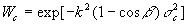
|
(31)
|
where sc2
is the mean square relative displacement (MSRD),
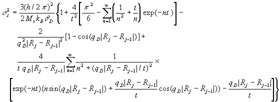
|
(32)
|
where Ms is the substrate or average atom atomic
mass, kB is the Boltzmann constant,
qD is the effective or
average atom Debye temperature,
t=qD/T,
T is the sample temperature in K, |Rj-Rj-1|
is the internuclear distance of the bond vector leading from the
site in a single scattering process, i.e. a' in Figure 3,
qD=wD/v is the
associated Debye wave vector, v is the velocity of sound which
is taken as constant in the Debye approximation,
wD is the cutoff frequency
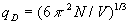
determined by
(6q2v3N/V)
1/3, N is the number of acoustic phonon modes in
volume V with the wave vector less than qD,
which equals the number of primitive cells, or usually the
number of atoms in volume V. So we have
|
(33)
|
This Debye-Waller attenuation factor has been adopted in equation
(32). Accounting for the surface atomic vibration is not as
straightforward. The relation between the MSRD and different
atomic masses has been given by Allen, Alldredge and Wette,
|
(34)
|
Correlating eqn (34) with (32), an effective surface atomic mass
is introduced such that
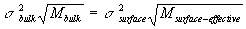
|
(35)
|
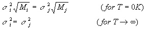
where Msurface-effective=Msurface if
T/qD<<1 or
Msurface-effective=Mbulk if
T/qD>1.
For T/qD ~ 1,
Msurface-effective
is allowed to vary between the surface and bulk atomic masses.
Inner potential correction
A photoelectron with energy E within the jellium medium will
have energy E-E0 in the vacuum far from the surface.
This loss of kinetic energy E0 may be related to a
potential barrier whose total height is V0,
defined as inner potential. The only energy relevant for the
scattering problem is the electron's kinetic energy when it
encounters a scattering potential. In photoemission, the
scattered electron is detected, and the inner potential
represents the physical kinetic energy lost when the electron
travels from the scattering potential edge to the detector.
This inner potential is approximately the sum of the work function
and the valence band-width.
The inner potential barrier will alter the photoelectron path.
We adopt a planar step barrier of height V0 just
outside the last row of ion cores. This is the usual first-order
model for the surface barrier, introduced for both low energy
photoemission and low-energy electron diffraction. The important
consequence of this model is a prediction that the emerging
photoelectron will be refracted in a direction away from the
surface normal in the manner of optical paths with

|
(36)
|
where V0 is the inner potential, Ein and
Eout are the electron kinetic energy inside and
outside the sample surface, kin and kout
the wave number inside and outside the surface,
qin and
qout the photoelectron
directions before and after refraction at the surface away from
the normal direction, see Figure 4. Substituting eqn (29) into
eqn (36), we obtain the inner potential correction formula
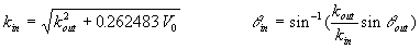
|
(37)
|
Presently there exist no generally acknowledged theoretical
or experimental inner potential data for any kind of element.
Hence it is treated as an adjustable parameter and fit to
experiment.
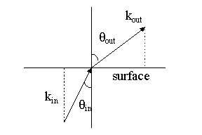
|
| Figure 4. Inner potential correction.
|
Instrumental angular averaging
The experimental apparatus for measuring photoemission intensities
has a small but finite angular resolution characterized by half
the angle subtended by the aperture at the source,
q in Figure 5. For small apertures,
q is the radius of the aperture
projected on a unit sphere so that the detected area is
q2.
The instrumental angular averaging due to this finite aperture
of the detector is done by summing the photoelectron intensities
over a grid of points on a circular aperture centered on the
nominal emission direction as defined by wave vector k.
We calculate photoemission intensities Ia,
Ib, Ic, Id and Ie
for five different directions (0,0)
(q,0)
(q,q/2)
(q,q)
(q,3q/2) and
(q,2q),
see Figure 5, and assume that the average intensity in each sector is the
average of the intensities at the three triangle corners. Then,
for example, in sector abc, the average intensity will be
Iabc=(Ia+Ib+Ic)/3.
For five point calculations, we obtain the average intensity
for a finite aperture of the detector

|
(38)
|
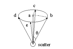
|
| Figure 5. Instrumental angular averaging;
q is the half aperture angle.
|