The Usage of MSCD Package

We have developed a program package to calculate and analyze the photoelectron diffraction intensity and their chi function using C++ with Object Oriented Programming (OOP) and the parallel computing technique Message Passing Interface (MPI). The code features the multiple scattering approach developed by Rehr and Albers, the TPP-2 inelastic mean free path formula developed by Tanuma, Powell and Penn, and the correlated temperature effect developed by Sagurton, Bullock and Fadley. The code simulates various kinds of experimental scanning modes, sample or analyzer rotation mechanisms, chi calculation algorithms, and their combinations. The scanned-angle calculation and built-in fitting procedure fits most analysis needs of photoelectron diffraction data. By avoiding any repeat calculations for identical events and identical path summing, the program speeds up the calculation dramatically compared with several other codes.

To run the program on different platforms, we split our package into two parts: a machine independent source code; and a machine-dependent source code. The same machine independent source code applies to both sequential and parallel computers. Using this structure, we have maximized code portability. Because the machine-dependent source code is relatively quite small (about 2 Kb), we can easily rewrite it to transfer the package to a new kind of computer.

The following diagram sketches the division of the code into a machine-independent part ("core program") and a machine-dependent part ("shell functions"). It gives examples of general calls in the core program that use machine-specific calls in the shell-functions part.

Parallel platforms		Sequential platforms
Cray T3E, COMPS		Cray J90, Sun workstation, IBM PC and Macintosh
Core Program (Machine Independent)		Shell Functions (Machine Dependent)
450 K source code, same for parallel or non-parallel		2 K source code for each platform
Use machine independent function calls everywhere		CPU time usage, and basic MPI functions
Example: int main(int argc, char **argv) { mpiinit(argc,argv); begcputime=processortime(); ... ... ... endcputime=processortime(); mpiend(); return(error); }		Example for Cray T3E: long processortime() { return(ta=times(&timebuf)); } void mpiinit(int *argc,char ***argv) { MPI_Init(argc,argv); } void mpiend() { MPI_Finalize(); }
Library functions, taken care of by C++ compiler Example: Void MPI_Init(argc,argv);

All the data files used or output by the mscd package programs are ASCII text file, having a unified mscd format data structure. This format consists of three parts.

1. The first part has only one line, i.e. the header line, including three integers, datatype, beginning-row, and line-numbers. Here, the three-digit datatype indicates what kind of data are in the file, beginning-row and line-numbers indicate the number of the first line counting from 1 for the head line and the number of total lines of the data body, i.e. the third part.
2. The second part, from the second line to the beginning-row of the data body, is a comment, introducing all the necessary information about the data.
3. The third part is the data body with a beginning line and line numbers indicated in the header line. The data are usually arranged in two or three columns, with spaces serving as the column delimiters.
4. We can put more comment lines after the third part.

Commonly used symbols and their definition in the mscd package:

Definition of the three-digit datatype of scanned-energy data file:

Date types of other files:

1. Prepare the potential data for all kinds of investigated atoms, in two columns. The first column is the radial distance r in Bohr unit (1 Bohr = 0.529167 Å), the second column is the corresponding potential multiplied by the radial distance, rV(r), in Bohr-Rydberg unit (1 Rydberg = 13.605 eV, 1 Bohr-Rydberg = 7.19932 ÅeV).
2. Use application program poconv to convert the potential data prepared in step 1) to mscd format potential data file.
3. Prepare input file, psrmin.txt, for phase shift and radial matrix element calculation.
4. Use application program psrm to calculate phase shift and radial matrix data if needed.
5. Prepare input file for photoelectron diffraction pattern calculation.
6. Prepare batch file, mscdin.txt.
7. Use application program mscd to perform the photoelectron diffraction pattern calculation.
8. If needed, prepare input file, holoin.txt, for hologram transformation.

Unit cell and cluster selection

The most complicated text file in mscd package is the input data file for a scanned-energy calculation. This file consists of non-structural parameters (like scanning mode, fitting mode, initial state, geometry, inelastic mean free path formula, temperatures, etc.) and structure parameters which determine the locations of atoms.

We define the surface structure by logical layers. A logical layer is a two-dimensional primitive lattice, or a two-dimensional Bravais lattice, which specifies the 2D-periodic array. A non-primitive physical layer must be divided into 2 or more primitive logical layers. Thus, a logical layer consists of all atoms with position vectors R of the form R(x,y,z) = m a(x,y) + n b(x,y) + R_layer-origin(x,y,z), where a and b are two-dimensional vectors, m and n range through all integral values which can be negative, zero as well as positive. R_layer-origin(x,y,z) is the location of the sample origin. The choice of two-dimensional vectors is not unique.

If a physical layer consists of two kinds of atoms, the layer can be divided into two logical layers. Each logical layer can have only one kind of atom. If the atoms in a physical layer are emitters, basically all the atoms in that layer are emitters, by periodic equivalence. Since the photoelectron diffraction intensities from different emitters are independent, we only need to consider a few emitters with different neighboring scatterers. In our code of photoelectron diffraction calculation, we take only one emitter for each logical layer: it is the atom which sits at that layer's origin. This way, even a primitive emitter layer may have to be divided into several logical layers, if more than one emitters have to be considered because of different neighboring atoms in three dimensions. This is the case, for instance, when an overlayer has a 2D structure with a superlattice or disorder, making substrate atoms translationally inequivalent: then the emission from these different atoms must be calculated independently and summed.

The ideal structure of a surface is infinite in extent in two dimensions and infinitely deep. To correctly represent photoelectron diffraction, we must in principle therefore take account of all scatterers within the surface. In practice, the contribution from a scatterer far from the emitter may be ignored. So we only need to choose a finite cluster including a few emitters and a finite number of scatterers, typically 100 atoms. In this program package, we use a cluster shape defined by a semi-ellipsoid: the profile as seen parallel to the surface is a semi-ellipse of minor axis r and major axis h; perpendicular to the surface it has as cross-section a circle of radius r. All the atoms within this semi-ellipsoid will be taken into account in the calculation. All the atoms outside this cluster are ignored. A bigger cluster selection will give a more accurate calculation, because of the smaller edge effect. But a bigger cluster calculation will take much more computation time and require a much larger computer memory. We have to make a compromise between cluster size and computation time. Typically, a cluster of 80 to 100 atoms is a reasonable choice, which requires 10 MB to 16 MB of random memory for single precision floating point computation, or double that for double precision floating point processing.

For testing purposes, we have two other alternative choices for the cluster. We can draw different circles or rectangles for each logical layer, all the atoms on that layer within that circle or rectangle will be considered.

Non-structural parameters

The non-structural input parameters are initial core-level, number of multiple scattering orders, R-A approximation order, scanning mode (description of energy scanning, polar angle scanning, azimuthal angle scanning, or hologram, i.e. two-angle scanning, using the same codes for the data type), detector instrumental half-aperture angle, photon polarization angles, Debye temperature, density and atomic weight for each kind of atoms, and number of valence electrons for the inelastic mean free path calculation.
See detail of those definitions.

In the current version, we only allow linearly polarized photons (other light polarizations are linear combinations of two perpendicular linear polarizations, and can be produced as such). The direction of photon polarization is described by its polar and azimuthal angles, theta(p) and phi(p). They are defined as the polar and azimuthal angles with respect to a reference direction, which depends on the rotation mechanism of the experimental geometry. If the surface normal direction is fixed (for example do not rotate sample, or only rotate it in azimuthal direction), the reference direction is this fixed surface normal. If the surface normal is not fixed (rotatable), in a reasonable experimental geometry, the analyzer must be fixed, then the reference direction is this fixed analyzer direction.

The photoemission intensity curves versus energy or angles consist typically of a series of diffraction peaks and troughs. To compare calculated with experimental intensities I, we have to remove the atomic partial cross section from intensities I₀, leaving only the oscillating part of the intensity, which we call chi function or c function.

chi = (I-I₀)/I₀

Because the free atom cross-section I₀ contains only very low frequency information, we will make little error at the structurally important frequencies if we approximate I₀ as the smooth part of I.

More specifically, in our MSCD program package, to extract this background I₀ from an energy-scanned or polar-angle-scanned curve, we fit it as a cubic spline function to both calculated and experimental intensity curves using the non-linear Marquardt fitting method. To make this spline function, we choose 3-5 initial data points of equal step as fitting parameters, which ensure a smooth background and have only very low frequencies. For an azimuthal-angle-scanned curve, because the cross-section along azimuthal direction can be thought as a constant, we just use the average of the intensities as the background I₀.

Although the multiple scattering theory can well reproduce the experimental photoemission intensity, the agreement is never perfect. To quantify the goodness of fit or to automatically fit structural parameters to the data, we introduce the reliability or R-factor. In our MSCD package, we use two reliability factors Ra and Rb, defined as follows together with a similar factor R:

R = sum_j(chi_cj - chi_ej)² / sum_j(chi_ej)²

R_a = sum_j(chi_cj - chi_ej)² / sum_j(chi_cj + chi_ej)²

R_b = sum_j(chi_cj² - chi_ej²) / sum_j(chi_cj² + chi_ej²)

These R-factors are related to the traditional Pendry reliability factor for used in LEED; chi_c is the calculated chi value, while chi_e is the experimental one, the sum index j is taken over all the corresponding data points for both curves. The first factor R is used by many groups, Ra is the factor used in our fitting procedure, Rb is a factor which tells us the quality of amplitude agreement. The largest effect on the overall amplitude of the chi function stems from the thermal vibration: thus, from the Rb value, we will have an idea how good the Debye temperature is.

In the complicated photoelectron diffraction theory, many parameters, such as temperature, inner potential, geometry and structural parameters, affect the photoemission intensity in a non-monotonous way. Thus, fitting may be the only effective method to perform the fitting of such parameters to experiment. A good reliability factor is then required to control the fitting process. In our MSCD package, we use the Ra factor, instead of R, to peform the fit, for the following reason.

For the best trial calculation, R and R_a are both small (<< 1.0). The amplitudes of calculated and experimental data are quite close, i.e.

R_a-best ~ R_best (for Rbest << 1.0)

For the worst trial calculation, the calculated intensity is irrelevant to the experimental curve. We would have

R_worst = 1 + A_try²/A_exp²
R_a-worst = 2.0

Here, Atry and Aexp are the average amplitude of the trial calculated and experimental intensity curves, respectively. Because Atry could be much less than Aexp in the fitting procedure while changing parameters, especially the Debye temperature, so we can write

R_worst = 1.0
R_a-worst = 2.0

Using the simplest single-scattering model of scanned-energy, chi can be written as

chi(k) = sum_j { A_j(k) cos[ k (R_j - R_j cos(theta_j) + phi_j ] }

where k is the wave vector, A_j the amplitude, R_j the bond length, theta_j the scattering angle, and phi_j the phase of the jth scattering event. Let us consider only one component with same frequency k but with different amplitudes and phases for the trial and experimental curves, namely

chi_c(k) = A_try cos( k x + phi)
chi_e(k) = A_exp cos ( k x )

R / R_worst = [ A_try² + A_exp² - 2 A_try A_exp cos (phi) ] / A_exp²
R_a / R_worst = [ A_try² + A_exp² - 2 A_try A_exp cos (phi) ] / [A_try² + A_exp²]

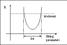
Here we found R_a/R_a-worst < R/R_worst. We know, once a trial R-factor is greater than one of the extreme worst cases, that the fitting procedure would fail to continue towards the best minimum. The next figure shows an R-factor plot versus the fitting parameters. Assuming A_try = A_exp, delta(phi) in the figure will be the available fitting range of phase phi in the above equation. Obviously, we hope phi to be as large as possible. From the above equation, we find phi = 120° if we use R as R-factor and assume A_try = A_exp, and phi is even smaller when A_try < A_exp. However, we can see that phi = 180° if we use R_a as the R-factor to monitor the fitting process. This is the reason we use R_a as the monitoring R-factor in our fitting procedure.

	Figure. R-factor plot versus fitting parameters. If a trial R-factor is greater than the worst case (irrelevant), the fitting procedure would fail to continue.

For a poorly-known system, we may have several structural parameters to fit, such as layer spacing, location of adsorbate atom, surface reconstruction, etc. Because the inner potential and Debye temperature are not well understood so far, we have to keep them adjustable, too. All these parameters influence the photoemission intensity in a complicated way. Changing any of them may introduce more than one local minimum. Therefore, a simple conventional fitting method would not be enough in most cases. In our code, we perform the fitting in a three-step process.

1. In the first step, we do a net search, in which calculations are made on a set of given grid points in fixed stepsize basis for each fitting parameter, and their R_a factor is monitored. This allows us to search a larger area, even if there are more than one local minimum. Ending this process, the best minimum and its parameters are chosen as the initial parameters of the next step.

2. In the second step, the program uses a downhill simplex method in multi-dimensions monitoring the R_a factor. This method requires only function evaluations, not derivatives. It is not very efficient in terms of the number of function evaluations that it requires. However, it may frequently be the best method to use if the figure of merit (here R_a factor) is "get something working quickly" for a problem whose computational burden is small. Once a trial calculation gives an R_a factor less than a given (input) tolerance, the downhill simplex loop will stop and transmit the best parameters to the next step.

3. In the third step, we use the non-linear Marquardt fitting method, which is the most refined search in our package. This method works very well in practice and has become a standard non-linear least-squares approach.